Analysis of 3D pointcloud

This tutorial explains:

• How to compute a persistence diagram from 3D pointcloud data
• How to visualize the diagram
• How to output birth-death pairs to a text file
• How to apply inverse analysis

These techniques are common for any pointcloud data, so you shoubd better to be familar with these features.

How to compute a PD

The target data is stored in pointcloud.txt. The file contains random 5000 points coming from 3D standard normal distribution. We analyze this data for exercise.

First of all, we display the data. First 10 lines are shown as below.

head pointcloud.txt

-1.688604987600753837e+00 5.699006029198190326e-01 -1.346186823505619579e+00
1.087144905453914845e+00 1.934202933045750861e+00 8.273916713882594198e-01
-1.157236831361657392e-01 -1.168206946858528328e+00 -3.994263428990901810e-01
-1.602174172538033403e-01 -8.626762802439005284e-01 1.188676117430170320e+00
5.613694793886953027e-02 -8.925811823166075465e-01 7.867005084945112303e-01
-3.121247358971382946e-01 -2.982206113960411131e-01 1.317235943833295453e+00
9.831752257585583132e-01 -2.465116319438791059e+00 -6.081245384492277584e-01
-7.600677459838747207e-01 -6.142993053684995264e-01 3.828101574633524518e-01
3.666431208906655304e-01 -4.606251408481700227e-01 1.759186989342665930e+00
3.009754635114507137e-01 5.049945721030327794e-01 1.429650286762043088e+00

There are three columns to represent 3D data.

Now we compute a PD. python3 -m homcloud.pc_alpha is used. We have a shortcut command whose name is homcloud-pc-alpha for convenience. You can also use this shortcut command.

python3 -m homcloud.pc_alpha -d 3 pointcloud.txt pointcloud.pdgm

Then a file named pointcloud.pdgm is generated. This file contains the information of PD. You should give the dimension of the data by -d 3. The input file path and the output file path are pointcloud.txt and pointcloud.pdgm.

How to visualize a PD

Here, we plot the PD. The following command plots the PD.

python3 -m homcloud.plot_PD -d 1 pointcloud.pdgm -o pointcloud-pd1.png

-d 1 means that 1st PD (corresponding to the ring structures) is plotted. If you want to plot the 2nd PD (corresponding to the cavities), please use -d 2. You can specify the path of output image by -o pointcloud-pd1.png. The following image is generated.

The display command shows an image in the environment of jupyter notebook with bash.

display < pointcloud-pd1.png

Nothing is shown except some grids around (0.0, 0.0). This is because many birth-death pairs are concentrated around (0.0, 0.0). Therefore, we change the colorbar to log-scale. -l option specifies log-scale. We also adjust the scale of X-axis and Y-axis. You can adjust by --aspect equal option.

python3 -m homcloud.plot_PD -d 1 -l --aspect equal pointcloud.pdgm -o pointcloud-pd1-log.png
display < pointcloud-pd1-log.png

Basically, a birth-death pair far from the diagonal corresponds to an "important" or "meamingful" ring structure. Therefore, a pair near (0.5, 0.7) possibly corresponds to the most meaningful ring structures in the pointcloud.

Now you should pay attention of X-axis and Y-axis. A textbook says that the X-axis and Y-axis means the radii of balls, but HomCloud uses the square of radii. $\sqrt{0.5} \simeq 0.7$ and $\sqrt{0.7} \simeq 0.84$ are the real radii. HomCloud uses the square mainly because of the internal implementation, but there is another reason that the square is more natural if an weighted pointcloud is used. If you want to use the radii instead of the square of radii, please use --no-square option to homcloud.pc_alpha.

Next, we zoom up the area around 0.0. By default, HomCloud plot the diagram to show all birth-death pairs. We can change the range of plotting by -x option.

python3 -m homcloud.plot_PD -d 1 -l -x "[0:0.1]" --aspect equal pointcloud.pdgm -o pointcloud-pd1-zoomup.png
display < pointcloud-pd1-zoomup.png

Of course, the data is random, there is no "typical" ring structures. But, the histogram is "typical" for a random pointcloud.

You can change the resolution of the histogram by -X option. The default resolution is 128x128. The below command plots the histogram whose resolution is 256x256.

python3 -m homcloud.plot_PD -d 1 -l -x "[0:0.1]" -X 256 --aspect equal pointcloud.pdgm -o pointcloud-pd1-zoomup.png
display < pointcloud-pd1-zoomup.png

In the above exercise, the histograms are saved into image files and the files are displayed by display command. We can also show the historam by the interactive interface of matplotlib if -o option is not given.

plot_PD_gui module is also available. This module provides advanced interactive user interface. You can change the range and resolution interactively from GUI. The following command invokes the GUI program.

python3 -m homcloud.plot_PD_gui -d 1 pointcloud.pdgm

Attribute Qt::AA_EnableHighDpiScaling must be set before QCoreApplication is created.

How to output the birth-death pairs in text format.

Here, we try to output the birth-death pairs as text data. If you want further analysis of PDs, this command is helpful.

# tail is used to show only 10 lines because the number of lines is quite large.
python3 -m homcloud.dump_diagram -S no -d 1 pointcloud.pdgm | tail 

0.5973638046166524 0.6105533327957627
0.5652198460841742 0.6333196314607091
0.5906213675656147 0.6399900554981125
0.6442572283186025 0.6455006374894877
0.6619166403896363 0.6636272756594286
0.6716352526485909 0.6731624171711277
0.4845143271980769 0.6955406657117916
0.699242025096557 0.6994652025551098
0.7400408653215168 0.7484476418235964
0.7997505082496258 0.800028497810961

The output has two columns. The first column show birth times and the second column has death times. The values are the square of radii. If you want to output the 2nd PD, please use -d 2 option instead of -d 1. The option -S no is explained later.

If you want to save the text into a file, please use -o option as follows. The following command saves the 1st PD into pointcloud-pd1.txt.

python3 -m homcloud.dump_diagram -S no -d 1 pointcloud.pdgm -o pointcloud-pd1.txt

Simple inverse analsys (birth simplex and death simplex)

Each birth-death pair in a PD corresponds to a ring or cavity in the orignal pointcloud. In fact, identifing such a structure is not a easy task. This kind of analysis is called inverse analysis. HomCloud has some tools for inverse analysis. In this section, a simple inverse analysis tool called "birth simplex" and "death simplex" is introduced. You can see these simplices by homcloud.dump_diagram module with -S yes option.

python3 -m homcloud.dump_diagram -S yes -d 1 pointcloud.pdgm -o pointcloud-pd1.txt
# Only first three lines are shown
head -n 3 pointcloud-pd1.txt

0.0005037159143533377 0.0005579705552885796 ((0.9509954988275516,-1.0068450361062282,0.5444291481244738),(0.9578267519847968,-1.0257637674912665,0.5845574329183165)) ((0.9509954988275516,-1.0068450361062282,0.5444291481244738),(0.9491853165615161,-1.0446271794013047,0.5530720162883241),(0.9578267519847968,-1.0257637674912665,0.5845574329183165))
0.0009259080093991961 0.0009586588306071996 ((-0.28508278742529314,0.18171712515275223,0.11312983987397246),(-0.33924144759564706,0.1933836037205496,0.08794323938926972)) ((-0.28508278742529314,0.18171712515275223,0.11312983987397246),(-0.3409101402063031,0.16848605635352581,0.09550916713739144),(-0.33924144759564706,0.1933836037205496,0.08794323938926972))
0.0010596423596121558 0.001129414564220647 ((0.5526278710732792,0.6042269908917515,-0.5658452971742082),(0.5738152766437832,0.5718181805421756,-0.5135066661702851)) ((0.5526278710732792,0.6042269908917515,-0.5658452971742082),(0.5738152766437832,0.5718181805421756,-0.5135066661702851),(0.5712305433890057,0.6264996091243692,-0.5476846170921237))

First two columns shows birth and death times. Next two columes shows birth and death simplices. Each row in third and fourth column is around by braces {...}.

The above output menas that the first line has the information about a birth-death pair (0.0005037159143533377, 0.0005579705552885796) and the corresponding ring structure appears when the edge connecting the following two vertices:

(0.950995498828,-1.00684503611,0.544429148124)
(0.957826751985,-1.02576376749,0.584557432918)

and the ring disappears when the triangle whose vertices are the following three points:

(0.950995498828,-1.00684503611,0.544429148124)
(0.949185316562,-1.0446271794,0.553072016288)
(0.957826751985,-1.02576376749,0.584557432918)

Normally death simplices are more important than birth simplices because the center of a death simplex is likely the center of the ring. The birth and death simplices are saved into pointcloud-pd1.txt and you can find the spatial distribution of rings by analyzing the file.

Advanced inverse analysis tool called optimal volume

An optimal volume, a powerful inverse analysis tool, is introduced in this section. Please see the paper by I. Obayashi for the details of optimal volume.

The following figure is the 1st PD shown above.

display < pointcloud-pd1-log.png

Now we analyze the birth-death pair near (0.5, 0.7) by using an optimal volume. homcloud.optvol module is available for that purpose. The following command computes the optimal volume corresponding the birth-death pair (0.5, 0.7). The degree is specified by -d 1 and the pair is specified by -x 0.5 -y 0.7. This moudle automatically finds the nearest birth-death pair and computes optimal volume of the pair. By using -P option, the volume is visualized by ParaView.

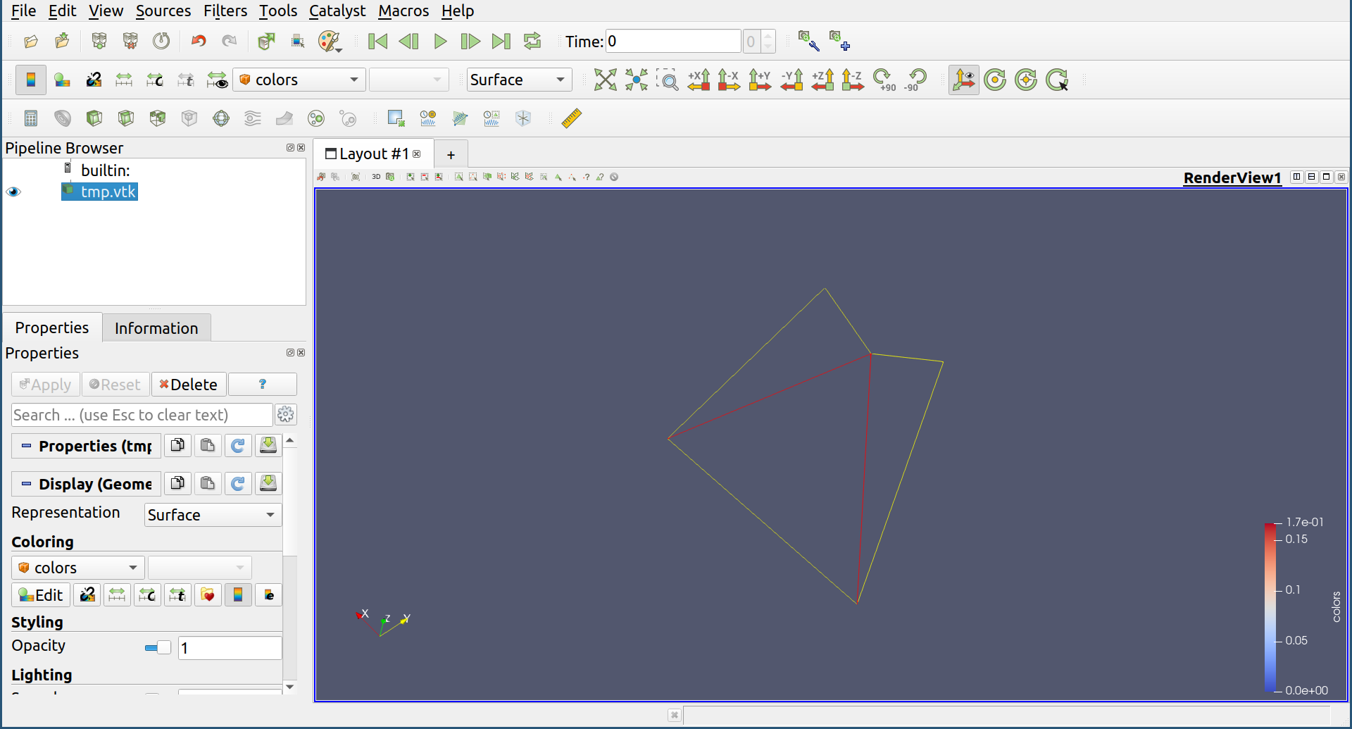
python3 -m homcloud.optvol -d 1 -x 0.5 -y 0.7 -P pointcloud.pdgm

By the above command, a paraview window is popped up. Please click the "Apply" button in the left panel to show. The green ring is the volume-optimal cycle, it is the ring that you want. Other information is also shown. For example, the red lines shows the internal volume of the ring.

You can save the information in json format by the following command.

python3 -m homcloud.optvol -d 1 -x 0.5 -y 0.7 -j optimal_volume.json pointcloud.pdgm

The information is saved into optimal_volume.json.

Probably you wander which is better, an optimal volume or birth / death simplices. An optimal volume have richer information but the computation cost is more expensive. I recommend that an optimal volume is usually used and if your data is huge and the computation cost is too expensive, it is better to use birth and death simplices.

This tutorail finish here.