Analysis of a 3D pointcloud

This tutorial explains:

1. How to compute a persistence diagram (PD) from a given a 3D pointcloud data
2. How to visualize the PD
3. How to extract each birth/death times
4. How to see the geometric origin of a birth-death pair

Since these analyses are common for any pointcloud data, this tutorial is helpful if you want to any kinds of pointclouds.

Computing a PD

The input data for this tutorial is sotred in pointcloud.txt. This file have 1000 points in a 3D space.

Now we try the analysis of the data.

First of all, we import some libraries.

import homcloud.interface as hc  # HomCloudのインターフェース
import numpy as np  # NumPy (数値配列)
import matplotlib.pyplot as plt  # Matplotlib (PDの可視化用)
%matplotlib inline
import pyvista as pv  # PyVista (3D可視化)

Change the backend of pyvista to trame. See https://docs.pyvista.org/user-guide/jupyter/index.html. If 3D visualization does not work well, please try to change 'trame' to 'panel'.

pv.set_jupyter_backend('trame')

Load the data by np.loadtxt.

pointcloud = np.loadtxt("pointcloud.txt")

Try to see the information of the pointcloud.

pointcloud.shape

(1000, 3)

The shape of the array is 1000x3, this means that the number of points is 1000, and each point is localed in the 3D Euclidean space.

np.min(pointcloud, axis=0), np.max(pointcloud, axis=0)

(array([0.00026274, 0.00100671, 0.00020878]),
 array([0.99997803, 0.9993682 , 0.99825316]))

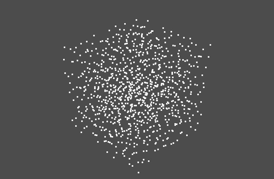
The points are distributed in the cube $[0, 1]\times[0, 1]\times[0, 1]$. Now we visualize the pointcloud by PyVista.

plotter = pv.Plotter()
plotter.add_mesh(pv.PointSet(pointcloud))
plotter.show()

Widget(value="<iframe src='http://localhost:34677/index.html?ui=P_0x7f9e617f2d70_0&reconnect=auto' style='widt…

The pointcloud is visualized as follows.

Now we compute a PD from the data. We use hc.PDList.from_alpha_filtration for that purpose. save_boundary_map option argument is required to compute optimal volumes later.

hc.PDList.from_alpha_filtration(pointcloud, 
                                save_to="pointcloud.pdgm",
                                save_boundary_map=True)

PDList(path=pointcloud.pdgm)

Then the file pointcloud.pdgm is created. This file contains all information about the PD.

Visualize a PD

Next, we plot the PD.

Load pointcloud.idiagram by hc.PDList.

pdlist = hc.PDList("pointcloud.pdgm")

The returned object has PDs of all degrees. We get the 1st PD by dth_diagram.

pd1 = pdlist.dth_diagram(1)

Then we construct a histogram from the 1st PD and plot the histogram. histogram method construct a histogram, then plot it by plot method.

pd1.histogram().plot()

This figure shows something at the bottom-left. This is because many birth-death pairs are concentrated around there.

Therefore, we change the colorbar from linear-scale to log-scale.

pd1.histogram().plot(colorbar={"type": "log"})

In 1st PDs, a birth time with a large lifetime (death - birth) corresponds a "meaningful" ring. Therefore, the ring corresponding the birth-death pair (0.0025, 0.008) is, in some sense, the most significant ring.

Here, we remark that HomCloud uses the squares of radii in the birth and death axes.
For example, for the birth-death pair (0.5, 0.7), the ring appear at radius $\sqrt{0.0025}=0.5$ and disappears at $\sqrt{0.008} \approx 0.09$. This is maily because of the internal implementation of HomCloud, but this is also because squares are better for weighted pointclouds (pointclouds with initial radii).

If you do not want to use squares, please use the argument no_squared=True when hc.PDList.from_alpha_filtration is called.

Next we investigate the PD around (0.005, 0.005). HomCloud automatically adjusts the range of a histogram to plot all birth-death pairs. We can change the range of a histogram by x_range argument of histogram method.

pd1.histogram((0, 0.01)).plot(colorbar={"type": "log"})

Of course, there is no meaningful information in the PD since the data is randomly generated. However, it is very helpful for you to know typical PDs for random data.

If you want to change the resolution of the histogram, please use x_bins argument of histogram method. The default value of x_bins 128, and this means that the resolution of histogram is 128x128. We change the resolution into 256x256.

pd1.histogram((0, 0.01), 256).plot(colorbar={"type": "log"})

These figures are plotted by using matplotlib, so we can save the figure by matplotlib.pyplot.savefig. The following code saves the figure into pointcloud-pd1.png.

pd1.histogram((0, 0.01), 256).plot(colorbar={"type": "log"})
plt.savefig("pointcloud-pd1.png")

The 2 dim PD is also visualized.

pd2 = pdlist.dth_diagram(2)

pd2.histogram().plot(colorbar={"type": "log"})

In the PD, there are some birth-death pairs whose birth time is larger than 0.0125 with large lifetimes (death times minus birth times).

Read birth times and death times

We can get birth/death times by births and deaths attributes of the pd object.

pd1.births

array([0.00140906, 0.00139591, 0.00134116, ..., 0.01572219, 0.01709659,
       0.01871588])

pd1.deaths

array([0.0015926 , 0.00164399, 0.00170775, ..., 0.0157662 , 0.01717465,
       0.01880101])

We can compute the lifetimes by the difference.

pd1.deaths - pd1.births

array([1.83534435e-04, 2.48078852e-04, 3.66588805e-04, ...,
       4.40061409e-05, 7.80638251e-05, 8.51306753e-05])

Now we plot the histogram of lifetimes by matplotlib.

plt.hist(pd1.deaths - pd1.births, bins=100);

; suppress the return value of plt.hist.

Inverse analysis of PD

Each birth-death pair in a PD corresponds to a topological structure such as a ring and a cavity. But it is not easy to find such a structure. Finding such a structure is called an "inverse analysis".

Here we use HomCloud's powerful inverse analysis tool. The following types of inverse analysis tools are available.

• Birth/Death simplices.
• Optimal Volume
• Stable Volume

Here we use the latest feature, stable volume. This solves the noise-sensitivity problem of optimal volumes. We examine the stable volume of the birth-death pair near (0.0025, 0.008).

We can use pd.nearest_pair_to to find the nearest birth-death pair to (0.0025, 0.008).

pair = pd1.nearest_pair_to(0.0025, 0.008)

This object is an instance of the class Pair, and the object has birth time and death time.

pair

Pair(0.0025623095880009357, 0.008135892057712315)

pair.lifetime()

0.005573582469711379

The following code computes the stable volume of the pair. 0.00005 means the scale of virtual noise. The first choice of this parameter is 1/10 -- 1/100 of the lifetime.

stable_volume = pair.stable_volume(0.00005)

boundary_points shows the coordinates of points in the ring structure.

stable_volume.boundary_points()

[[0.24041004740553085, 0.3620263927982651, 0.3938519814000714],
 [0.07850470821281752, 0.31832538225761675, 0.2726051865809148],
 [0.1255383953826733, 0.0800900311964785, 0.7190957020829821],
 [0.1252375238953729, 0.20843145021582987, 0.37381081780757186],
 [0.27896903483481006, 0.2900038108788685, 0.3853792732744701],
 [0.11968719444459341, 0.46213675229879714, 0.6086047255929676],
 [0.10439142042970573, 0.12004955606294554, 0.3999294686167837],
 [0.07478379187666995, 0.1318144315592794, 0.6167927456566142],
 [0.241996106473225, 0.4429189262369284, 0.4639170406136188],
 [0.12423094383664512, 0.3622394365995112, 0.6448082172747804],
 [0.19443369660602383, 0.2643008696498902, 0.7685550494906768],
 [0.41898602615433533, 0.44362916692289767, 0.3710002303374377],
 [0.12195279248515212, 0.003239458152972219, 0.6061209669659768],
 [0.21608561791517278, 0.2918069725141198, 0.3219258262415402],
 [0.1894939883612946, 0.03095999913576697, 0.6762565272706147],
 [0.0708147888171643, 0.05566245889432686, 0.6142169362499716],
 [0.39171929078549805, 0.4405548898038244, 0.288435385498083],
 [0.21062788160417378, 0.11633529728096403, 0.5162505592185838],
 [0.3166872139448015, 0.38348372951946463, 0.33415602643779374],
 [0.3806980910779977, 0.4089441782551778, 0.43539259723846135],
 [0.17739556404702383, 0.10003158291956527, 0.43755332223623955],
 [0.1563951908464587, 0.13629542421604657, 0.594303189697284],
 [0.15814254898557367, 0.44579878013749064, 0.4799628611505681],
 [0.17887993848973416, 0.42554668220768377, 0.6217943706156428],
 [0.09845847975583133, 0.26404248130005237, 0.7778474474038211],
 [0.3373945662185728, 0.46415106121781036, 0.4856613355037861],
 [0.08346167978435703, 0.26153343284444097, 0.3241366037151565],
 [0.08561651425017891, 0.42297356026275923, 0.528205350556188],
 [0.12886238414379725, 0.17512618876757002, 0.7438074952407614],
 [0.16660019888277078, 0.33716865816694763, 0.30111066188327684],
 [0.32035651808142795, 0.4751033316678963, 0.34029734006837487],
 [0.18678772331743787, 0.34044366488617717, 0.7226556446102448]]

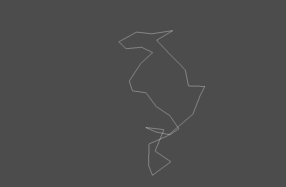
We find that the ring have 39 points. The method boundary shows the connections between points.

Finally, we visualize the optimal volume in 3D space.

pl = pv.Plotter()
pl.add_mesh(stable_volume.to_pyvista_boundary_mesh())
pl.show()

Widget(value="<iframe src='http://localhost:34677/index.html?ui=P_0x7f9e616df760_1&reconnect=auto' style='widt…

A ring is shown as follows.

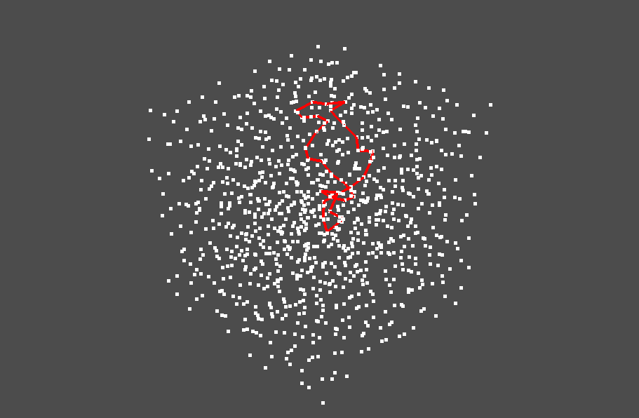
We will use pyvista's functionality to overlay the pointcloud on the ring. We can adjust the line width and the line color using pyvista.

pl = pv.Plotter()
pl.add_mesh(pv.PointSet(pointcloud))
pl.add_mesh(stable_volume.to_pyvista_boundary_mesh(), color="red", line_width=4)
pl.show()

Widget(value="<iframe src='http://localhost:34677/index.html?ui=P_0x7f9e6030d960_2&reconnect=auto' style='widt…

The ring is visualized as follows. You can rotate and zoom up/down the figure.

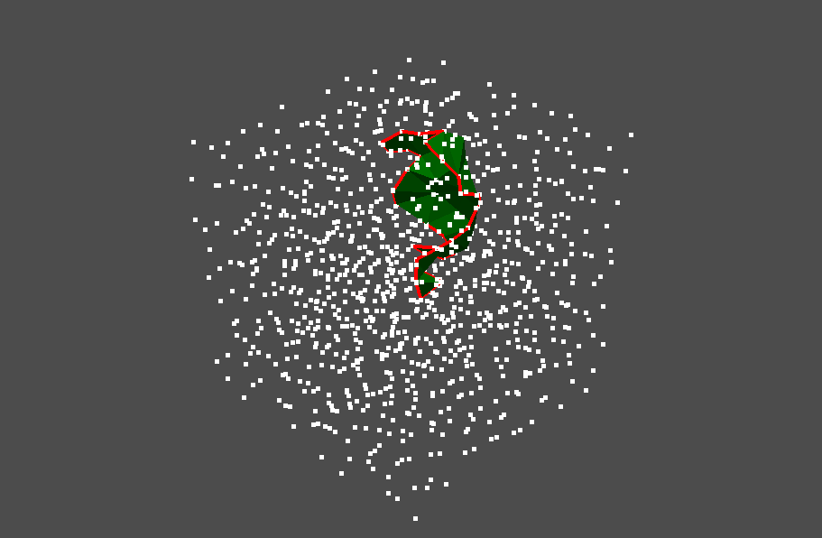
You can also visualize the internal area of the stable volume (the area enclosed by the ring).

pl = pv.Plotter()
pl.add_mesh(pv.PointSet(pointcloud))
pl.add_mesh(stable_volume.to_pyvista_boundary_mesh(), color="red", line_width=4)
pl.add_mesh(stable_volume.to_pyvista_volume_mesh(), color="green")
pl.show()

Widget(value="<iframe src='http://localhost:34677/index.html?ui=P_0x7f9e616dea70_3&reconnect=auto' style='widt…

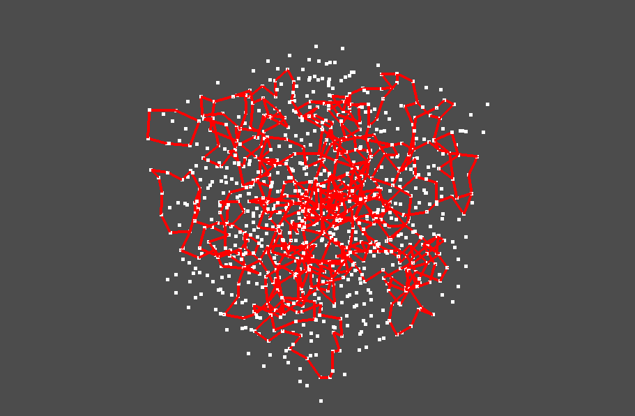
Now we try to visualize multiple stable volumes. We focus on the birth-death pairs whose birth times are less than 0.005 and death times are larger than 0.006.

pairs = [pair for pair in pd1.pairs() if pair.birth_time() < 0.004 and pair.death_time() > 0.006]

len(pairs)

54

The number of pairs is 54. Now the stable volumes for these pairs are computed. Since the number is a bit large, the computation time is quite long. To reduce the time, we use cutoff_radius parameter of stable_volume method. This parameter restricts the simplices used in the computation. The simplices are restricted in the sphere whose radius is the given value. Now cutoff_radius is 0.5. This radius is estimated by the half of the length of the side of the cube.

%%time
stable_volumes = [pair.stable_volume(0.00005, cutoff_radius=0.5) for pair in pairs]

CPU times: user 9.18 s, sys: 118 ms, total: 9.3 s
Wall time: 11 s

pl = pv.Plotter()
for stable_volume in stable_volumes:
    pl.add_mesh(stable_volume.to_pyvista_boundary_mesh(), 
                color="red", line_width=4)
pl.add_mesh(pv.PointSet(pointcloud))
pl.show()

Widget(value="<iframe src='http://localhost:34677/index.html?ui=P_0x7f9e601e04c0_4&reconnect=auto' style='widt…

Inverse analysis for 2 dim PD

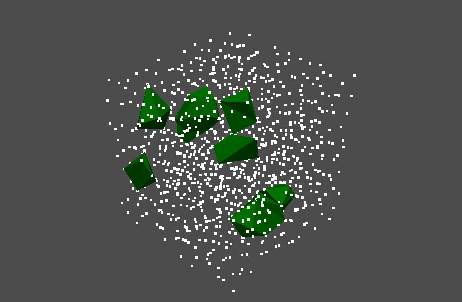
We also visualize the voids in the same way. We focus on pairs whose birth time is larger than 0.0125 and whose lifetimes are larger than 0.0005.

pairs = [pair for pair in pd2.pairs() if pair.birth_time() > 0.0125 and pair.lifetime() > 0.0005]

stable_volumes = [pair.stable_volume(0.000005) for pair in pairs]

pl = pv.Plotter()
for stable_volume in stable_volumes:
    pl.add_mesh(stable_volume.to_pyvista_boundary_mesh(), color="green")
pl.add_mesh(pv.PointSet(pointcloud))
pl.show()

Widget(value="<iframe src='http://localhost:34677/index.html?ui=P_0x7f9e51ac70d0_5&reconnect=auto' style='widt…

We can find some large voids in the pointcloud.

Appendix (Advanced topics)

In this section, some advanced topics such as vertex naming, optima 1-cycles, PHTrees, initial radii, and BackgroundPlotter are introduced.

Vertex naming

Up to now, vertex information retrieved by boundary_points and other methods has been in XYZ coordinates. While this may be convenient in many cases, we sometime want to use information such as "the 4th point" or "the 12th carbon atom". Vertex naming funcitonality allows for such a request.

Any string is allowed as a name. You can give the same name to different vertices (HomCloud will distinguish between vertices with the same name internally.)

Here, we have 1000 points and name the points "000", ..., "999".

names = [f"{n:03d}" for n in range(1000)]

We can name points by passing the list of names to vertex_symbol argument of from_alpha_filtration.

hc.PDList.from_alpha_filtration(pointcloud, vertex_symbols=names, save_boundary_map=True, save_to="pointcloud-with-names.pdgm")

PDList(path=pointcloud-with-names.pdgm)

Now we again compute a stable volume and examine the vertices of the volume. We can get the list of names of the vertices on the ring using boundary_points_symbols instead of boundary_points.

pd1 = hc.PDList("pointcloud-with-names.pdgm").dth_diagram(1)
pair = pd1.nearest_pair_to(0.0025, 0.008)
stable_volume = pair.stable_volume(0.0005)
stable_volume.boundary_points_symbols()

['392',
 '147',
 '154',
 '297',
 '170',
 '939',
 '442',
 '957',
 '832',
 '065',
 '580',
 '581',
 '582',
 '972',
 '080',
 '721',
 '480',
 '870',
 '872',
 '491',
 '236',
 '237',
 '750']

Optimal 1-cycle

Internally stable volume is calculated using linear programming, and when the number of points is large, the computation cost is quite high. To speed up the computation, HomCloud has some special mechanisms.

When analyzing a 1D PD, the tool called "optimal 1-cycle" is available. An optimal 1-cycle differs from the optimal/stable volume of the same birth-death pair, and the optimal/stable volume is more reliable than the optimal 1-cycle. However, the optimal 1-cycle can be computed much faster than the corresponding optimal/stable volume. If the number of points is large, please consider using optimal 1-cycles.

As in the example above, the optimal 1-cycle of the closest birth-daeth pair to (0.0025, 0.008) is calculated as follows.

pair = pd1.nearest_pair_to(0.0025, 0.008)
optimal_1_cycle = pair.optimal_1_cycle()

We visualize the cycle as follows.

pl = pv.Plotter()
pl.add_mesh(optimal_1_cycle.to_pyvista_mesh(), color="red", line_width=4)
pl.add_mesh(pv.PointSet(pointcloud))
pl.show()

Widget(value="<iframe src='http://localhost:34677/index.html?ui=P_0x7f9e51ed34f0_6&reconnect=auto' style='widt…

The following code retrieves the information about the edges of the ring.

optimal_1_cycle.path()

[[[0.1255383953826733, 0.0800900311964785, 0.7190957020829821],
  [0.1894939883612946, 0.03095999913576697, 0.6762565272706147]],
 [[0.1255383953826733, 0.0800900311964785, 0.7190957020829821],
  [0.12886238414379725, 0.17512618876757002, 0.7438074952407614]],
 [[0.12886238414379725, 0.17512618876757002, 0.7438074952407614],
  [0.09845847975583133, 0.26404248130005237, 0.7778474474038211]],
 [[0.19443369660602383, 0.2643008696498902, 0.7685550494906768],
  [0.09845847975583133, 0.26404248130005237, 0.7778474474038211]],
 [[0.19443369660602383, 0.2643008696498902, 0.7685550494906768],
  [0.18678772331743787, 0.34044366488617717, 0.7226556446102448]],
 [[0.18678772331743787, 0.34044366488617717, 0.7226556446102448],
  [0.2422121988843836, 0.4155487622456445, 0.7075748545403898]],
 [[0.3058423940248698, 0.3873355905611001, 0.6845908848342269],
  [0.2422121988843836, 0.4155487622456445, 0.7075748545403898]],
 [[0.3058423940248698, 0.3873355905611001, 0.6845908848342269],
  [0.3756708152548601, 0.4044688174747033, 0.6376955289875823]],
 [[0.42889440234947107, 0.4185878889153811, 0.5784790134722813],
  [0.3756708152548601, 0.4044688174747033, 0.6376955289875823]],
 [[0.42889440234947107, 0.4185878889153811, 0.5784790134722813],
  [0.4598816637670946, 0.4162817757882945, 0.49121522961841546]],
 [[0.47167872450123804, 0.3563222306553614, 0.4586659808644902],
  [0.4598816637670946, 0.4162817757882945, 0.49121522961841546]],
 [[0.47167872450123804, 0.3563222306553614, 0.4586659808644902],
  [0.4643529555106557, 0.38891409104439234, 0.37758039548286215]],
 [[0.41872842706632685, 0.3117355628197983, 0.36357591323139904],
  [0.4643529555106557, 0.38891409104439234, 0.37758039548286215]],
 [[0.41872842706632685, 0.3117355628197983, 0.36357591323139904],
  [0.39907517145005755, 0.2831943114569727, 0.4368217260059085]],
 [[0.34941504868714357, 0.20455144955416626, 0.4210171084082195],
  [0.39907517145005755, 0.2831943114569727, 0.4368217260059085]],
 [[0.34941504868714357, 0.20455144955416626, 0.4210171084082195],
  [0.296676557056482, 0.1310208804226647, 0.43046852751189457]],
 [[0.296676557056482, 0.1310208804226647, 0.43046852751189457],
  [0.2927591672470917, 0.11598883729155451, 0.5038453999131621]],
 [[0.21062788160417378, 0.11633529728096403, 0.5162505592185838],
  [0.2927591672470917, 0.11598883729155451, 0.5038453999131621]],
 [[0.21062788160417378, 0.11633529728096403, 0.5162505592185838],
  [0.1563951908464587, 0.13629542421604657, 0.594303189697284]],
 [[0.1563951908464587, 0.13629542421604657, 0.594303189697284],
  [0.07478379187666995, 0.1318144315592794, 0.6167927456566142]],
 [[0.0708147888171643, 0.05566245889432686, 0.6142169362499716],
  [0.07478379187666995, 0.1318144315592794, 0.6167927456566142]],
 [[0.0708147888171643, 0.05566245889432686, 0.6142169362499716],
  [0.12195279248515212, 0.003239458152972219, 0.6061209669659768]],
 [[0.1894939883612946, 0.03095999913576697, 0.6762565272706147],
  [0.12195279248515212, 0.003239458152972219, 0.6061209669659768]]]

PHTrees

When analyzing a 2D PD, PHTrees (persistence trees) are available. PHTrees compute the information about 2D PH very fast using the mathematical idea of duality.

By passing save_phtrees=True to from_alpha_fitratlion, HomCloud computes PHTrees together with PDs.

hc.PDList.from_alpha_filtration(pointcloud, 
                                save_to="pointcloud-phtrees.pdgm",
                                save_phtrees=True,
                                save_boundary_map=True)

PDList(path=pointcloud-phtrees.pdgm)

Read PHTrees as follows.

phtrees = hc.PDList("pointcloud-phtrees.pdgm").dth_diagram(2).load_phtrees()

As in the above example, we examine birth-death pairs where birth > 0.0125 and lifetime > 0.0005. PHTrees have a forest (multiple trees) structure internally, and each birth-death pair corresponds to a node in a tree.

stable_volumes = [node.stable_volume(0.000005) for node in phtrees.all_nodes if node.birth_time() > 0.0125 and node.lifetime() > 0.0005]

Visualize them as follows.

pl = pv.Plotter()
for sv in stable_volumes:
    pl.add_mesh(sv.to_pyvista_mesh(), color="green")
pl.add_mesh(pv.PointSet(pointcloud))
pl.show()

Widget(value="<iframe src='http://localhost:34677/index.html?ui=P_0x7f9e4b9e07f0_7&reconnect=auto' style='widt…

The result is the same as the above example.

You can retrieve the information about the shapes using boundary_points, boundary, and other methods.

stable_volumes[0].boundary_points()

[[0.6994453732085671, 0.13144153221118793, 0.5796928995428492],
 [0.601928672387627, 0.08671998624231247, 0.6583244074235682],
 [0.6994366874462885, 0.002942826575932589, 0.8357930347813906],
 [0.7794027918486173, 0.20026894822385644, 0.7191885213983096],
 [0.7064811805219977, 0.0026801020745949033, 0.5743802347904137],
 [0.8393149713230158, 0.04786549991547495, 0.6049694308550129],
 [0.8709165597839585, 0.12038179501110158, 0.6840309300141862]]

In addition, you can also analyze the trees strucures of PHTrees. For details, see the PHTrees section of the HomCloud API manual.

Initial radii

Suppose you wish to analyze data in which particles have their own scale, for example, atomic configuration data consisting of multiple types of atoms. In that case, you can analyze the data reflecting their radii. Whe $i$-th atom has a radius of $r_i$, this analysis can be performed by preparing an array $w = [r_0^2, \ldots, r_{N-1}^2]$. The HomCloud rule requires squared radii.

In the following example, the initial radius of the first 500 particles out of 1000 is 0.01, and the radius of the remaining 500 particles is 0.05.

weights = np.concatenate([np.full(500, 0.01 ** 2), np.full(500, 0.05 ** 2)])

hc.PDList.from_alpha_filtration(pointcloud, weight=weights, 
                                save_boundary_map=True, save_to="pointcloud-weights.pdgm")

PDList(path=pointcloud-weights.pdgm)

pd1 = hc.PDList("pointcloud-weights.pdgm").dth_diagram(1)
pd1.histogram().plot(colorbar={"type": "log"})

If the initial radius is positive, birth and death times may be negative. This is a situation where the sphere is shrunk from the initial radius.

The radius increasing rule is $\sqrt{\alpha + r_i^2}$.

BackgroundPlotter

Visualization with pyvsita + jupyter notebook can sometimes be underperforming. In such cases, you can use the BackgroundPlotter from pyvistaqt.

If you feel the integrated visualization with jupyter is difficult to use and the visualization on a separate window is better, BackgroundPlotter is helpful.

Note that BackgroundPlotter cannot coexist with a regular pyvista Plotter It is recommended to use only one of them.

import pyvistaqt as pvqt

pl = pvqt.BackgroundPlotter()
pl.add_mesh(pv.PointSet(pointcloud))
pl.show()